Runoff is a crucial component of the hydrologic cycle. Understanding how much water will be conveyed to hydraulic structures, such as storm drains, pipes, culverts, or water bodies, is critical to designing adequate stormwater infrastructure. For this reason, it is essential that hydrologic and hydraulic (H&H) modelers accurately depict the relationship between rainfall and runoff. There are several methods for modeling stormwater runoff. A common example of an empirical method for calculating runoff is the SCS Curve Number Method. Several software programs account for the spatial variability of stormwater runoff.
Traditionally, hydrologic and hydraulic modeling have been separate exercises, each requiring a distinct modeling program. For example, HEC-HMS performs hydrologic calculations and generates a hydrograph that can be used as an upstream boundary condition for a HEC-RAS model. However, rain-on-grid modeling combines hydrologic and hydraulic modeling by applying rainfall directly to a 2D mesh. The runoff from that cell is then dependent on various parameters of the cell, such as rainfall depth, infiltration losses, Manning’s n value (roughness), surrounding slope, and water levels, as well as the cell’s area. The following blog post describes rain-on-grid modeling using the Hydrologic Engineering Center’s River Analysis System (HEC-RAS).
Comparison of HEC-RAS Rain on Grid Modeling and HEC-HMS
The Hydrologic Engineering Center’s Hydrologic Modeling System (HEC-HMS) is a program developed by the United States Army Corps of Engineers to model hydrologic processes. The predecessor of HEC-HMS, HEC-1, performs similar computations. Some engineers still prefer to use HEC-1 because it offers more control in certain aspects. However, HEC-1 does not have a graphical user interface (GUI).
Before HEC-RAS, a separate hydrologic model was developed using HEC-HMS or HEC-1. The output of such models would serve as the input for a hydraulic model developed in HEC-RAS. Although HEC-RAS rain-on-grid modeling enables H&H modelers to capture both hydrology and hydraulics in a single modeling software, the two programs do not perform calculations in the same manner. The table below outlines the differences between rain-on-grid modeling in HEC-RAS and hydrologic modeling in HEC-HMS.
| Calculation Description | HEC-RAS 2D | HEC-HMS |
| Infiltration is the process of water entering the soil profile through the ground surface. | Infiltration Calculation Methods Available: – Deficit and Constant – SCS Curve Number – Green and Ampt | Infiltration Calculation Methods Available: – Deficit and Constant – Exponential – Green and Ampt – Gridded Deficit Constant – Gridded Green and Ampt – Gridded SCS Curve Number – Gridded Soil Moisture Accounting – Initial and Constant – Layered Green and Ampt – SCS Curve Number – Smith Parlange – Soil Moisture Accounting |
| Routing | Water is conveyed through cell faces | Basins are routed together using generalized calculations for each basin |
| Hyetographs which depict rainfall intensity over time. | – The user can only input a single hyetograph per flow area | – Can develop hyetographs from rainfall depth input |
| Results | – Flows, velocities, and flow depths are calculated for each cell face. | – Generates a single hydrograph output per model element |
Why Rain-On-Grid Modeling?
Many engineers and modelers are accustomed to developing hydrologic models well. With numerous robust hydrologic modeling tools available, why bother with rain-on-grid? There are some reasons to apply precipitation to your HEC-RAS 2D mesh. Rain-on-grid modeling can be a suitable approach for large areas, particularly when exact flow patterns are unknown. Many modelers will run a rain-on-grid HEC-RAS model, extract the flow hydrographs for their area of interest, and develop a more detailed/refined hydraulic model for a select area. Some of the advantages of rain-on-grid modeling include:
- There is no need to delineate drainage areas, which can be a difficult exercise for flat areas.
- The ability to model cross-catchment flows that occur during large storm events.
- A simplified modeling process since the hydrology and hydraulics are combined.
Rain-on-grid modeling does have its drawbacks. The first drawback is that a high-quality digital elevation model (DEM) is required, and this DEM must cover the entire catchment area. As a result, the run times can be somewhat lengthy. The large terrain datasets and lengthy run times associated with rain-on-grid modeling also tend to increase file sizes. This can make it challenging to share and store model files with reviewers and other team members.
It is also worth noting that a debate exists among hydrologists regarding the accuracy of rain-on-grid. Rain-on-grid modeling often results in shallow flow depths. It is recommended that calibration be used to verify the accuracy of parameters such as Manning’s n. Because HEC-RAS 2D does not allow for depth-varying Manning’s n, it can be challenging to account for both shallow flow depths and deeper flows associated with typical Manning’s n values for channels. Other parameters, such as infiltration and rainfall, can also introduce significant uncertainty into a model. Another potential issue related to accuracy is that a rain-on-grid model is unlikely to account for stormwater features not represented in coarser terrain data. Such features may include ditches, small detention ponds, piping, or curb and gutter.
Adding a Precipitation Boundary Condition
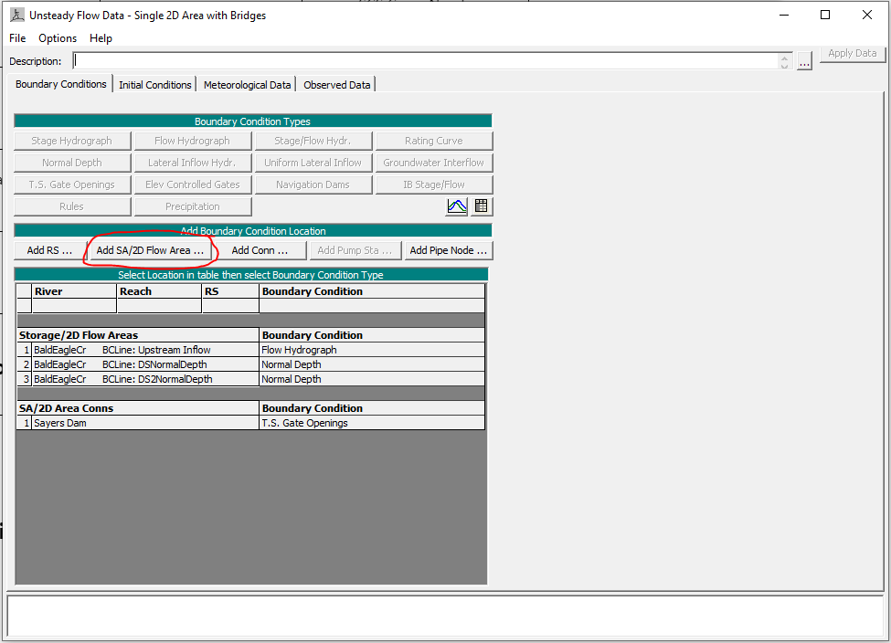
To apply rainfall to a two-dimensional (2D) mesh in HEC-RAS, first navigate to the Unsteady Flow Data Editor.
Next, click the Add SA/2D Flow Area button, which is circled in red in the image below.
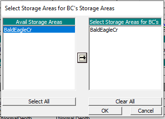
Select the applicable 2D flow area and use the arrow in the middle of the screen to move it to the right side of the box. Finally, click Ok.
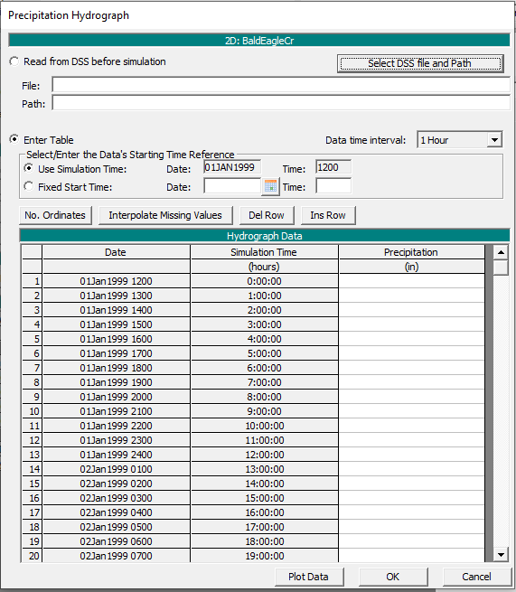
Next, click the Precipitation boundary condition button. The window shown in the image below will appear. Simply populate the Precipitation column with your hyetograph. It is important to note that the precipitation values you enter in the Precipitation Hydrograph dialog box should represent excess precipitation unless your terrain has an infiltration grid associated with it.
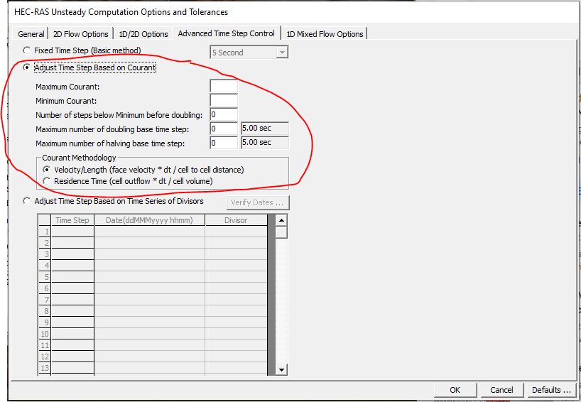
It is essential to proceed with caution when adjusting the time step based on the Courant Number. This is because HEC-RAS will examine your highest velocities, which may not be present in your channel if your 2D mesh includes areas with steep slopes. As a result, you may need to run your 2D model for much longer than you would if you used a fixed time step.
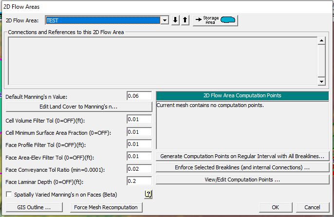
Adjusting the 2D Flow Area Properties for Rain on Grid Modeling
The default values may not provide sufficient detail to accurately depict the very shallow depths that need to be calculated when preparing a rain-on-grid HEC-RAS model. Thus, the default tolerances shown in the table below should be decreased by one or two orders of magnitude. This will produce cell face property tables that compute volume at more discrete intervals so that shallow depths are not overly simplified.
Adding Infiltration to a Rain-on-Grid HEC-RAS Model
HEC-RAS allows the user to create an Infiltration Layer in RAS Mapper for the purpose of estimating losses. The Infiltration Layer defines the method used to estimate losses from a precipitation event. The methods available in HEC-RAS include the SCS Curve Number Method, the Deficit and Constant Method, and the following methods are provided below.
Data required for the SCS Curve Number Method:
- Curve number for each land cover/hydrologic soil group combination.
- Initial abstraction ratio for land cover/hydrologic soil group combination.
- Minimum infiltration rate for each land cover/hydrologic soil group combination.
Data required for the Deficit and Constant Method:
- Maximum deficit (in).
- Initial deficit (in).
- Potential evapotranspiration (ET) (in/hr).
- Potential infiltration rate (in/hr).
Data required for the Green-Ampt Method:
- Wetting front suction (in).
- Saturated hydraulic conductivity (in/hr).
- Initial soil water content.
- Saturated soil water content.
- Soil Potential Evapotranspiration (ET) (in/hr).
You can import an Infiltration Layer created outside of HEC-RAS. To create an Infiltration Layer in RAS Mapper, the user must first generate a land cover dataset and a S Mapper, and how to use those layers to create an Infiltration Layer that can be used in your rain-on-grid model.
Creating a Land Cover Dataset
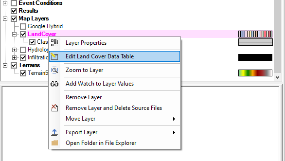
To create an infiltration layer in HEC-RAS, you must first create a land cover dataset. Creating a land cover dataset is also helpful for defining Manning’s n for each land cover type. You can create your own land cover dataset in GIS and import the resulting shapefile or raster layer into HEC-RAS. Alternatively, you create a land cover dataset in HEC-RAS using data from the National Land Cover Dataset (NLCD). This method is useful if you are modeling a large area and it is impractical to delineate land cover manually using aerial imagery. After importing the NLCD data, use Classification Polygons to further refine your land cover dataset. After importing your land cover dataset and finalizing the Classification Polygons, right-click your land cover data and select Edit Land Cover Table as shown in the image below.
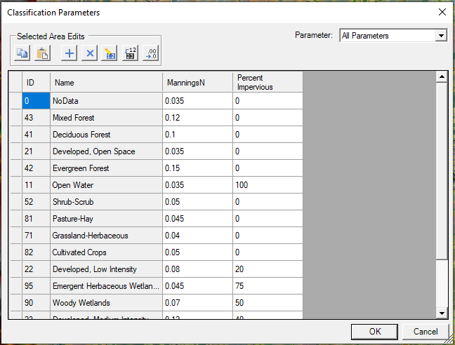
The following table will appear. Populate the Manning’s n column of the table. The Percent Impervious column is optional depending on what infiltration method you select for your model.
Creating a Soils Layer
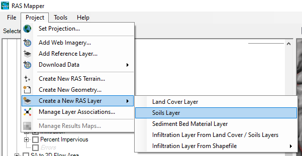
Next, you will need to add a Soils Layer to your HEC-RAS model that will classify soils into hydrologic soil groups (HSG). In the United States, this information can be obtained from the Natural Resources Conservation Service (NRCS) Soil Survey Geographic (SSURGO) Database. Simply download the soil data associated with your study area from the NRCS Web Soil Survey. Then select Create a New RAS Layer and Soils Layer from the Project menu in RAS Mapper (see image below).
Then navigate to the geodatabase (.gdb) file you downloaded from the Web Soil Survey. After the data loads, use the dropdown menu to select whether your Soils Layer will be based on hydrologic soil group, texture, or both.
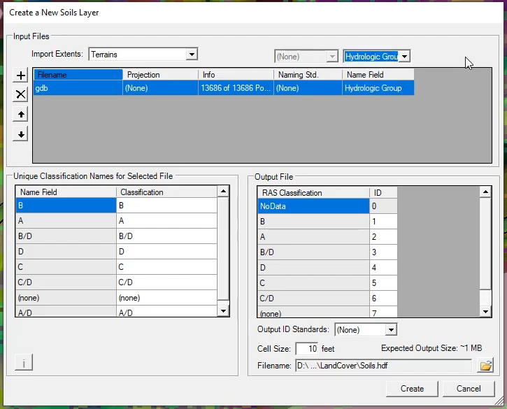
Finally, click the Create button and HEC-RAS will generate a raster layer of the soils dataset.
Creating the Infiltration Layer
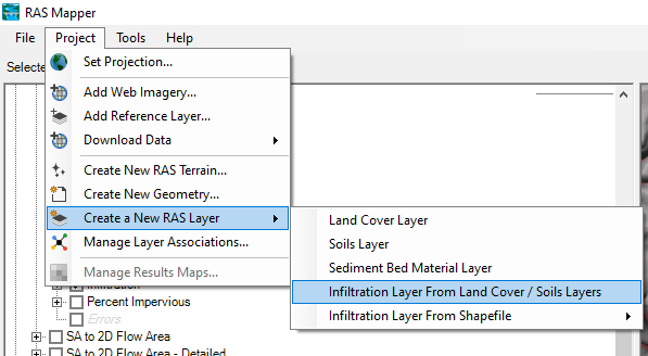
Finally, to create the final infiltration layer, select Create a New RAS Layer and Infiltration Layer from Land Cover / Soils Layers from the Project menu in RAS Mapper (see image below).
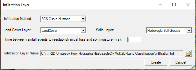
The dialog box shown below will appear. You can then select the applicable infiltration method, Land Cover Layer, and Soils Layer. You do not have to select both a Land Cover Layer and Soils Layer. The time between rainfall events to establish initial loss and soil moisture is also an option. It is useful if you have a multi-peaking event. Finally, click the Create button to generate the infiltration layer.
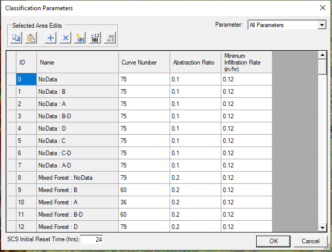
After creating the infiltration layer, right-click your infiltration dataset in RAS Mapper and click Edit Infiltration Data Table as shown below.
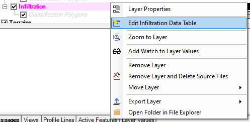
A table like the one below will appear and allow you to populate relevant infiltration parameters.
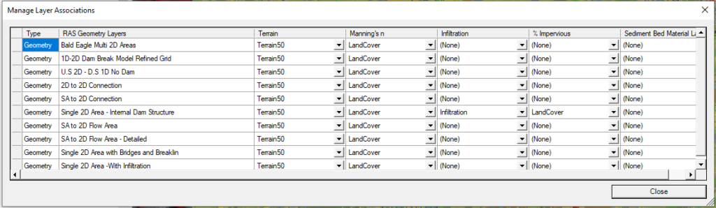
Specify Geometry Associations
After creating the datasets described above, right-click Geometries in RAS Mapper and click Geometry Associations. The following table will appear. Use the dropdown arrows to associate your land cover and infiltration layers with the appropriate geometry file.
Adding Gridded Precipitation Data to HEC-RAS
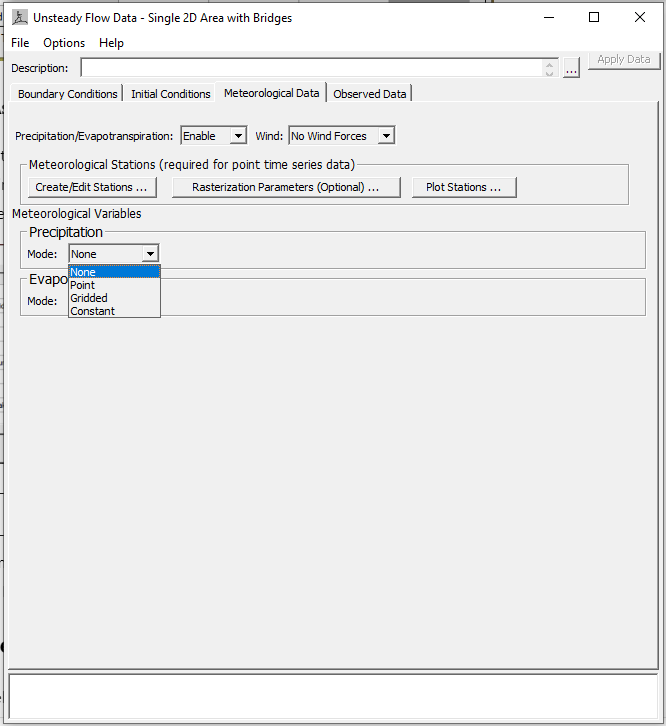
After preparing the geometry files as described above, it is time to work on preparing your flow data in the Unsteady Flow Data Editor. In the Unsteady Flow Data Editor, there is now (in HEC-RAS version 6) a tab called Meteorological Data. By default, Precipitation/Evapotranspiration is disabled. Simply, use the dropdown menu to enable the meteorological variables. Some options will then appear under Precipitation. The following sections will describe each of the three modes available (e.g., Point, Gridded, Constant).
Point
You can also add precipitation data to your HEC-RAS model as point gauge data. HEC-RAS interpolates the point gauge data and converts it to a gridded format. To add this kind of precipitation data to your HEC-RAS model, first, click on Create/Edit Stations to enter the name and coordinates of each gage as shown below (Figure 4-12 from the HEC-RAS 2D User’s Manual).
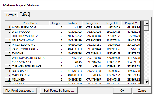
Next, select the interpolation method (Thiessen Polygon, Inverse Square of the Distance, Inverse Distance Squared (Restricted), Peak Preservation). Finally, upload the DSS file for each rain gage.
Gridded
The Gridded option enables you to enter precipitation files in either DSS format or raster format. The DSS option is helpful if you used another program to get the precipitation data into that format. The United States Army Corps of Engineers offers a free program that can assist you in doing this. It is called HEC-MetVue. You can check out that program using the link below.
If the GDAL Raster Files option is selected, . These are National Weather Service (NWS) file formats for NWS gridded data.
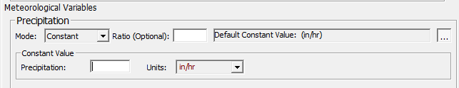
Constant
The Constant option allows the user to enter a constant rainfall intensity as shown below.
Evapotranspiration and Wind Data
Evapotranspiration (ET) data are only used for the Deficit, Constant, Green-Ampt infiltration methods. Even then, it is optional and only valid when modeling dry periods between rainfall events. ET is added to HEC-RAS in a manner similar to precipitation. It can be entered as gridded data, point gauge data, or just a constant rate.
Wind forces can be incorporated in both 1D and 2D unsteady flow modeling. Like precipitation and ET data, wind data (speed and direction) can be entered as either gridded data or point gauge data.
Adjusting Rendering Mode for a Rain-on-Grid Model
After running your model with a Precipitation boundary condition, you may notice that the model results appear disjointed. To give your model’s results a smooth appearance, it is essential to adjust the render mode. In HEC-RAS version 6.2, you can do this by navigating to RAS Mapper and selecting Options under the Tools menu. Then click Render Mode under Project Settings.
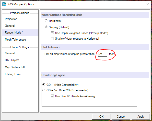
Simply adjust the Plot Tolerance to only plot water depths greater than the value indicated. You may also want to consider checking Use Depth-Weighted Faces (“Precip Mode”). This option gives cell faces with deeper water depths more weight than those with shallower water depths. It is important to note that changing the way that adjusting the options in Render Mode does not change the HEC-RAS results/computations. Rather, it just adjusts the way the results are displayed.
Limitations of Rain-On-Grid Modeling
The following section will help you understand some of the limitations of rain-on-grid modeling in HEC-RAS.
All models are wrong, but some are useful
George E. P. Box
Terrain Data
Like a 2D hydraulic model, rain-on-grid models that contain terrain data with a coarser spatial resolution may not accurately capture the hydraulics associated with smaller terrain features and, therefore, will not be as accurate as a model with better terrain data. It is also important to ensure that the modeler adds breaklines to capture roadway crowns and berms that may influence flow patterns.
Computation Time
Rain on grid HEC-RAS models takes a very long time to run because every cell within the 2D mesh is wetted by rainfall. You also need to include the entire catchment area to generate accurate results, and the simulation time must be sufficiently long to capture the time of concentration for the entire drainage area.
Limited Infiltration Calculations
HEC-RAS can model infiltration over a 2D flow area. However, infiltration is subtracted from the precipitation hyetograph. The program is not capable of performing infiltration calculations based on water depth. HEC-RAS can estimate infiltration using three methods: the Deficit and Constant Loss method, the SCS Curve Number Method, and Green-Ampt.