HEC-RAS Computation Options and Tolerances for Unsteady Flow Modeling

Unsteady flow modeling tends to be more complex and time-consuming than steady flow modeling. Instabilities become more of an issue, and addressing these instabilities is both an art and a science. Unfortunately, many modelers end up spending hours tweaking their crashing model only to discover that they needed to change just one setting to fix the problem. Understanding the options available in HEC-RAS will save you time and frustration, as familiarity with the program’s workings will enable you to address instabilities more effectively. The good news is that learning about these options does not require weeks of training. Setting aside a few hours to study the program’s options will significantly enhance your HEC-RAS unsteady flow modeling skills and ultimately save you time. I’m sharing the following blog post with you in the hope that it will be of use, as it provides an overview of the computation options and tolerance settings available for unsteady flow modeling in HEC-RAS.

Locating The HEC-RAS Unsteady Flow Modeling Computation Options and Tolerances

To find the HEC-RAS Unsteady Computation Options and Tolerances dialog box, first, navigate to the Unsteady Flow Analysis editor (click the icon that looks like a stick figure running up a hill). Once the Unsteady Flow Analysis editor pops up, select Options from the dropdown menu and click “Computation Options and Tolerances.” In the current version of HEC-RAS (6.3 at the time this blog post was written), the HEC-RAS unsteady flow computation options and tolerances are organized into the following tabs:

General,
2D Flow Options,
1D/2D Options,
Advanced Time Step Control, and
1D Mixed Flow Options.

The following sections of this article will describe the options available on each tab. It is worth noting that this blog post provides an overview of these options. For more details on how a particular choice affects your hydraulic model, refer to the HEC-RAS User’s Manual, which is available online.

General Tab

First, I will discuss the options available in the General tab (see screenshot below). This article will not include a description of every option available in HEC-RAS. Instead, I will discuss the settings I find most helpful for stabilizing unsteady flow models. For example, I will not discuss Wind Forces in this blog post as I have never had a reason to change the default. If you are interested in learning more about this option, refer to Chapter 2 of the HEC-RAS Version 6.0 Hydraulic Reference Manual for a detailed explanation of the various wind drag equations available in the program.

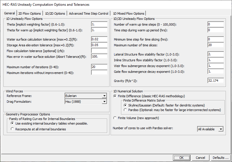
1D Unsteady Flow Options – Theta

When my hydraulic model experiences instability issues, I begin by examining the theta value, which is only applicable to 1D unsteady flow modeling. Theta is a weighting factor HEC-RAS uses to solve unsteady flow equations. The user can enter values between 0.6 and 1.0 for theta. A theta value of 0.6 is more accurate but less stable. In contrast, a theta value of 1 is more stable but less accurate. The general wisdom in hydraulic modeling is to start with simple models and gradually build complexity. For this reason, HEC has set the default theta value to 1. However, as you stabilize your model, I recommend lowering the theta value to achieve greater accuracy.

HEC-RAS also allows the user to establish a theta value for warm-ups, which represents the runtime that occurs before the actual simulation. In this case, HEC-RAS continues to use the entered theta value to solve the unsteady flow equations, but only during a different part of the simulation. I’ll talk about HEC-RAS model warm-ups in more detail later in this article.

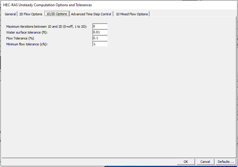
1D Unsteady Flow Options – Water Surface and Storage Area Tolerances

HEC-RAS uses water surface and storage area tolerances to solve the partial differential equations for the conservation of mass and momentum. The program goes through an iterative process to solve these equations. As a result, HEC-RAS has to make a few assumptions for specific parameters when it begins performing the hydraulic computations. The program then uses these guesses and results in the equation itself. After solving an iteration of these hydraulic calculations, HEC-RAS compares its guess to the actual result. The difference between those two values is calculated as an error. A more significant difference is associated with a higher number of errors. HEC-RAS tracks this error as it iterates through the solutions. If the calculated error exceeds the value specified in the unsteady flow options and tolerances, HEC-RAS will attempt another iteration to find an acceptable solution. By increasing the storage area tolerance or water surface tolerance, you make it easier for HEC-RAS to find a solution and proceed to the following calculation. However, it is essential to recognize that increasing these tolerances can lead to a more significant potential for error to accumulate over time and space, due to the nature of the partial differential equations governing the conservation of mass and momentum. This is why the program only allows you to increase the water surface calculation tolerance and storage area elevation tolerance to 0.2 feet.

The Max error in water surface solution represents the water surface error that will cause the program to stop running if it is exceeded. The default value is 100 ft.

It should be noted that, by default, the flow calculation tolerance is not used by HEC-RAS unless the user enters a value.

1D Unsteady Flow Options – Maximum Iterations

The maximum number of iterations options represents the number of times HEC-RAS will iterate through calculations to find an answer. The default value is 20 times.

Warm-Up Settings

As previously mentioned, warm-ups are simulation time that occurs before the “real” simulation begins. Specifically, a warm-up is a period of constant discharge added to the beginning of the run before the “real” simulation begins. In this way, it can be thought of as “negative” time. Warm-ups are useful for working out potential issues associated with initial conditions and help in generating smoother hydrographs. Warm-ups are particularly useful for quasi-steady models. It should be noted that you will not see the output from a warm-up period unless you change the settings to view it. The following sections will discuss the settings that apply to warm-ups.

Number of Warm-Up Time Steps

Users have the option to run more time steps (0 to 100,000). In previous versions of HEC-RAS, users could only run up to 40 warm-up time steps.

Warm-Up Time Step

It is sometimes necessary to use a time step that is smaller than the one used in the unsteady flow simulation. A smaller time step enables HEC-RAS to identify instabilities associated with the initial conditions before commencing the actual simulation. The default in HEC-RAS is to use the same time step as the unsteady flow simulation. This occurs if the warm-up time step box is left blank.

Time Slicing

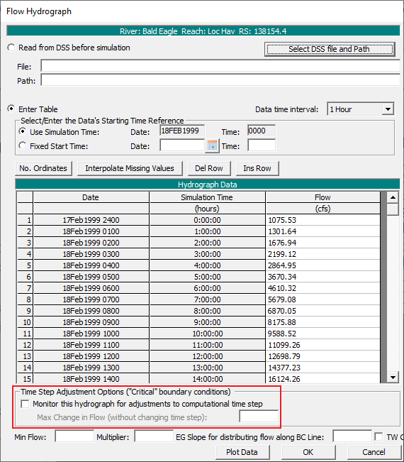
The time-slicing settings are associated with settings entered in the boundary conditions of the Unsteady Flow Editor (see the red outline on the screenshot below). If you check the “Monitor this hydrograph for adjustments to computation step” box and enter a value in the “Max Change in Flow” box, HEC-RAS will “slice” the hydrograph in areas where the inflow hydrograph (shown under the Flow column above the red outline in the screenshot below) changes by at least the amount indicated by the “Max Change in Flow” box.

Although the settings in the Unsteady Flow Data Editor control whether HEC-RAS slices the inflow hydrograph, the way HEC-RAS slices parts of the hydrograph where the change in flow exceeds the value in the “Max Change in Flow” box is controlled by the settings shown in the screenshot below (see red outline). HEC-RAS will not allow a slice that results in a time step below the minimum time step for time slicing, and the program won’t slice the inflow hydrograph more times than indicated by the maximum number of time slices box. It should be noted that the setting indicated by the red box below is strictly tied to an inflow hydrograph only if you have the appropriate box checked in the unsteady flow editor.

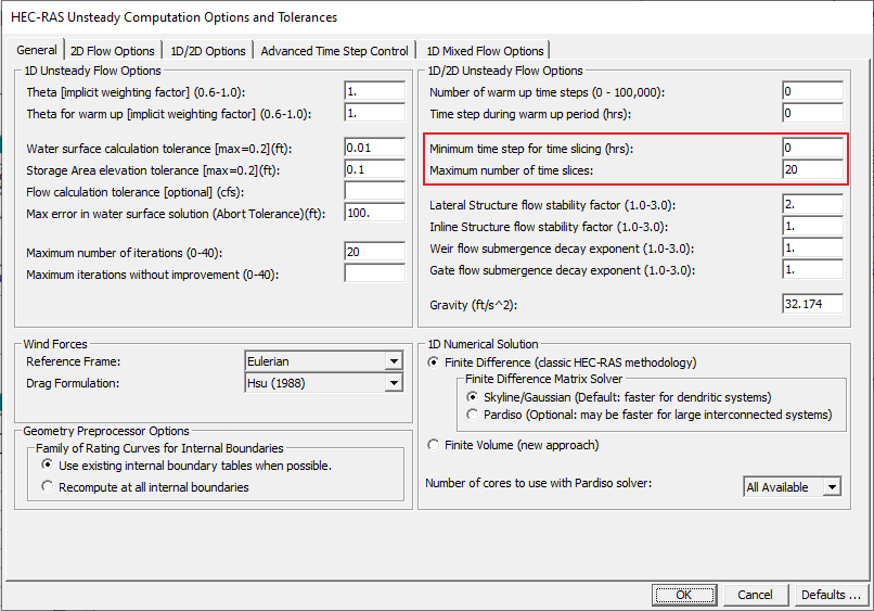
Stability Factors

Stability factors are similar to theta in that a larger value corresponds to better stability. A value of one corresponds to less stability but more accuracy. In contrast, a value of three is associated with more stability but less accuracy. If you are observing oscillations in your outflow hydrograph and your time step is low, consider increasing the stability factor to mitigate or eliminate the oscillations at the lateral or inline structure.

1D Numerical Solution

The default numerical solution solver is Skyline/Gaussian. I have not tried other options. If you want to learn about the other solvers, I recommend checking out the HEC-RAS model documentation, which is available on the HEC website. I also tend to keep the default value for “Number of cores to use with Pardiso solver.” I will discuss this option for 2D later in the article.

2D Flow Options

The 2D Flow Options tab will consist of a column of default options and a column for each 2D area in your geometry file. If a user changes the default options, any 2D areas added to the model after the change will have the new default options. In most cases, it is simpler to leave the default values alone and change the settings of each 2D area as necessary. Many of the settings are similar to those in 1D, but they are applied to 2D models. However, the default water surface tolerance in 2D is 0.01 ft instead of 0.02 ft (1D). The most important setting to understand in this tab is the equation set. The full momentum equations (SWE) are more accurate than the Diffusion Wave, but they result in longer run times and are prone to more instabilities. This is because Diffusion Wave is ultimately a simplification of the full shallow water equations (SWE). HEC has set the default equation set to Diffusion Wave, as they aim to encourage modelers to start with simplicity and gradually build complexity as they develop their models. In some cases, using the SWE may not significantly impact the model results. However, it is a good practice to run your final model using the SWE. For most applications, the SWE-ELM option is suitable. SWE-EM is used for near-field hydraulics.

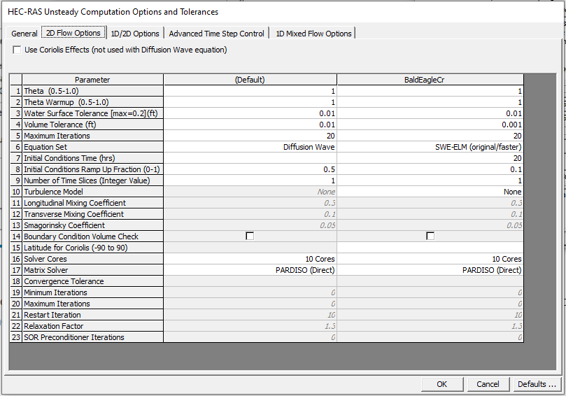
The Boundary Condition Volume Check can be helpful when your geometry includes features that have water flowing from one 2D area into another model element, such as two areas connected by an SA/2D area connection or a 1D reach flowing into a 2D area over a lateral structure. If the upstream feature begins to run out of water as the model simulation progresses, this setting ensures that HEC-RAS does not extract more water than what is available. Simply checking this box can prevent model errors, oscillations, or even crashes that result from inadequate water supply in a given time step. This option is particularly useful when running a dam break simulation, where the hydraulic model represents a situation in which water is flowing out of an upstream reservoir due to a dam failure.

At the top of the 2D Flow Options tab, users have the option to check a box that ensures that the model accounts for Coriolis Effects. Coriolis effects are generally not a significant concern. Unless you are modeling a very large reservoir or bay, checking this box is unlikely to significantly impact the results of your model. If you do choose to use the Coriolis Effects option in your 2D hydraulic model, enter the latitude of your project area in row 15. The value entered for latitude will only be used if the box at the top is checked and if you use the SWE.

HEC-RAS allows you to tell the program how to distribute tasks over the processing cores on your computer. All Available Cores is the default option. If you have a fancy computer with more than eight cores, this option can significantly improve the run times for large models with hundreds of thousands of cells. However, using too many cores can have a detrimental effect on smaller models, as HEC-RAS may spend more time distributing tasks to different cores rather than performing calculations. I do not have extensive experience with this option, as I have only run HEC-RAS models on standard computers rather than supercomputers with 32 cores. If you have a supercomputer or very powerful computer set aside for modeling, this may be a setting worth considering.

The default Matrix Solver is PARDISO. In previous versions of HEC-RAS, this was the only option. Now users can choose between PARDISO, SOR, and FGMRES-SOR. Most modelers still use the PARDISO option because it is the most stable. Once you have built a stable model, try out the iterative options to decrease run times. Just keep in mind that if you decide to use one of the “fancier” matrix solver options, the program will require you to enter some extra parameters (e.g., Minimum Iterations, Maximum Iterations, SOR Relaxation Factor, and Preconditioner Iterations).

1D/2D Options

If you encounter errors when connecting a 1D and 2D area, try increasing the number of iterations (first box). During a model simulation, the 1D and 2D “sides” share information such as stage or flow. A mismatch of these values results in errors and/or instabilities. By increasing the number of iterations, you are giving the program more chances to find a solution at the sub-time step level. As you can imagine, this can significantly slow down your model. It is also worth noting that the settings in the 1D/2D Options tab also apply to situations where 2D areas are connected by an SA/2D Area Connection.

Increasing the number of iterations at a 1D/2D connection should be considered a tool for identifying the underlying issues affecting your model. This setting should not be viewed as a “fix” for an unstable model.

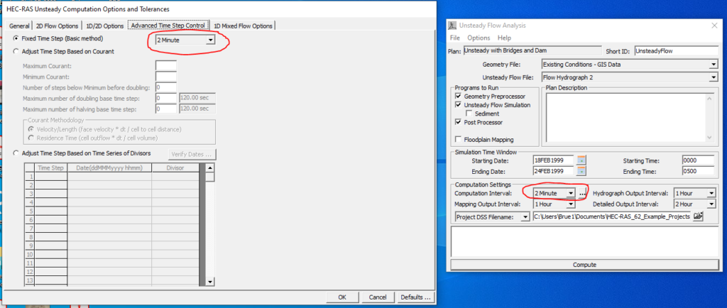
Advanced Time Step Control

The time step shown in the Advanced Time Step Control tab of the HEC-RAS Unsteady Computation Options and Tolerances dialog box (left side in the screenshot below) will be the same value as the computation interval shown in the Unsteady Flow Analysis window (right in the screenshot below). If the user changes the time step in one window, the computation interval will update in the other location.

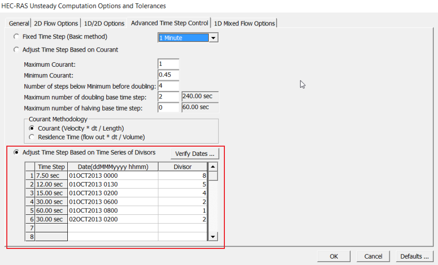
The option to Adjust the Time Step Based on Courant is helpful in cases where you are running a hydraulic model, particularly during the peak of a storm event, when a small time step is required. Rather than using a small time step for the entire simulation, the user can use the Courant option to make the model run faster while still ensuring a smaller time step is used during the flashy parts of the input hydrograph. However, it is essential to recognize that HEC-RAS requires additional computations to determine the Courant number. For this reason, adjusting the time step based on the Courant number will not significantly improve your run times. This is especially true if your model has underlying issues, such as cell sizes that are significantly smaller than necessary.

Many modelers find that the Adjust Time Step Based on Time Series of Divisors is a much more effective way to control your model. For this option, the user specifies the time step during a particular period during the model simulation. The screenshot below shows an example of input data for this option. The time step for each interval is equal to the Fixed Time Step number (1 minute in the example below) divided by the value entered in the Divisor column. It is worth noting that the numbers entered in the Divisor column must be whole numbers, or integers.

1D Mixed Flow Options

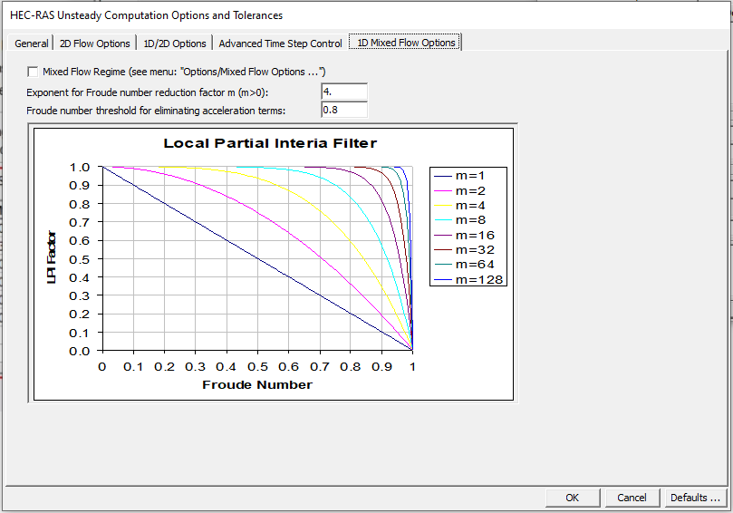
There is a common misconception that the mixed flow option allows you to run both subcritical and supercritical flows. However, this is not the case. This option is a method that HEC-RAS uses to stabilize hydraulic models when approaching critical depth. This option is commonly used for dam break modeling where there is a significant amount of local acceleration due to steep wave fronts associated with dam breaks. This local acceleration can cause errors and even model crashes. Using this setting can alleviate this problem. When modelers use the Mixed Flow Regime setting, HEC-RAS will monitor the Froude number throughout the model simulation. When the Froude number starts to get close to one, the HEC-RAS will multiply the local acceleration term (also known as the Local Partial Inertia (LPI) Factor) by the numbers on the y-axis of the chart. It is worth noting that some agencies may not accept models that utilize the 1D Mixed Flow Options tab.